| Score | Frequency | |
|---|---|---|
| 1 | 10 | 5 |
| 2 | 20 | 8 |
| 3 | 30 | 7 |
| 4 | 40 | 10 |
Statistics
1 Data
Let’s begin with the most fundamental concept in statistics, which is Data.
1.1 Categorical data and Quantitative data
Categorical data
Data that can be grouped by specific categories
Categorical values may be:
Binary – where there are only two distinct options, e.g. Subscribed vs Not Subscribed.
Ordinal – where the categories suggest a ranked order, e.g. Customer Satisfaction Level: Poor, Fair, Good, Excellent.
Nominal – where categories are labels without inherent order, e.g. Preferred Ice Cream Flavor: Chocolate, Vanilla, Strawberry.
The numbers help us represent the categories in code, but only ordinal values carry a meaningful sequence. For binary and nominal, the numbers are just labels with no mathematical relationship implied.
→ A categorical variable is a variable with categorical data.
NotePractice problem: Which of the following is an example of an ordinal categorical variable?
A. Type of fruit: Apple, Banana, Orange
B. Subscription status: Subscribed, Not Subscribed
C. Customer satisfaction level: Poor, Fair, Good, Excellent
D. Eye color: Blue, Brown, Green
TipSolution
C. Ordinal data has a meaningful order like Poor to Excellent
NotePractice problem: Which of the following describes nominal categorical data?
A. Education level: High School, College, Graduate
B. Preferred ice cream flavor: Chocolate, Vanilla, Strawberry
C. Pain level: Mild, Moderate, Severe
D. Employment status: Employed, Unemployed
TipSolution
B. Nominal data are labels without any inherent ranking or order
Quantitative Data
Data that use numeric values to indicate how much or how many are
Quantitative values can be:
Discrete - where values are distinct and countable, often whole numbers, eg: the number of books in the library.
Continuous - where values can take on any number within a range, including decimals, eg: the weight or height of a person.
→ A quantitative variable is a variable with quantitative data.
NotePractice problem: Which of the following is an example of discrete quantitative data?
A. Height of a basketball player
B. Number of pets someone owns
C. Temperature in a classroom
D. Time spent reading a book
TipSolution
B. Discrete data are countable whole numbers — like how many pets someone has
NotePractice problem: Which of the following represents continuous quantitative data?
A. Weight of watermelons in lb
B. Number of books on a shelf
C. Number of goals scored in a game
D. Books on a shelf
TipSolution
A. Continuous data can include fractions and decimals. Weight can vary smoothly across values.
1.2 Frequency, Relative Frequency, Cumulative Frequency
Frequency distributions are the foundation of data analysis - they help you organize and understand your data by showing patterns and trends. Think of them as different ways to count and display information from surveys, experiments, or observations.
1.2.1 Frequency
Frequency distribution: A tabular summary of data showing the number (frequency) of observations in each of several nonoverlapping categories or classes.
1.2.2 Relative Frequency
Relative frequency: shows the proportion of total responses each category represents. \[\text {Relative Frequency} = \frac{\text{Frequency of a class}}{\text{Total number of observations}}\]
Relative frequency distribution: A tabular summary of data showing the fraction or proportion of observations in each of several nonoverlapping categories or classes.
NotePractice problem
If a survey of 100 people shows that 25 prefer tea, what is the relative frequency of tea preference?
TipSolution
Frequency of class that prefers tea: 25
Total number of observations: 100 \[\text{Relative frequency of tea preference} = \frac {25}{100} \] \[\text{Relative frequency of tea preference} = 0.25 \]
1.2.3 Cumulative Frequency
Cumulative frequency distribution: A tabular summary of quantitative data showing the number of data values that are less than or equal to the upper class limit of each class. We can understand it as answering the question “How many up to this point?””
Test score example:
Below 60: 5 students (cumulative: \(5\))
Below 70: 8 students (cumulative: \(5 + 8 = 13\))
Below 80: 15 students (cumulative: \(13 + 15 = 28\))
Below 90: 12 students (cumulative: \(28 + 12 = 40\))
Cumulative relative frequency distribution: A tabular summary of quantitative data showing the fraction or proportion of data values that are less than or equal to the upper class limit of each class. Cumulative relative frequency runs totals as fractions or percentages instead of raw numbers
Same test scores as percentages:
Below 60: 12.5% of students
Below 70: 32.5% of students
Below 80: 70% of students
Below 90: 100% of students
NotePractice problem
Given the following data of scores and their frequencies, what is the cumulative frequency and cumulative relative frequency of those scores?
TipSolution
Calculating cumulative frequency
\(\text{Cumulative frequency of score 10 } = 5\)
\(\text{Cumulative frequency of score 20 } = 5 + 8 = 13\)
\(\text{Cumulative frequency of score 30 } = 5 + 8 + 7 = 20\)
\(\text{Cumulative frequency of score 40 } = 5 + 8 + 7 + 10 = 30\)
Calculating relative frequency
\(\text{Total observation of score} = 5 + 8 + 7 + 10 = 30\)
\(\text{Relative frequency of score 10} = \frac{5}{30} = 0.17\)
\(\text{Relative frequency of score 20} = \frac{8}{30} = 0.27\)
\(\text{Relative frequency of score 30} = \frac{7}{30} = 0.23\)
\(\text{Relative frequency of score 40} = \frac{10}{30} = 0.33\)
Calculating cumulative relative frequency
\(\text{Cumulative relative frequency of score 10} = 0.17\)
\(\text{Cumulative relative frequency of score 20} = 0.17 + 0.27 = 0.44\)
\(\text{Cumulative relative frequency of score 30} = 0.17 + 0.27 + 0.23 = 0.67\)
\(\text{Cumulative relative frequency of score 40} = 0.17 + 0.27 + 0.23 + 0.33 = 1\)
Frequency and Cumulative frequency distribution table
| Score | Frequency | Cumulative Frequency | Relative frequency | Cumulative Relative Frequency | |
|---|---|---|---|---|---|
| 1 | 10 | 5 | 5 | 0.17 | 0.17 |
| 2 | 20 | 8 | 13 | 0.27 | 0.44 |
| 3 | 30 | 7 | 20 | 0.23 | 0.67 |
| 4 | 40 | 10 | 30 | 0.33 | 1 |
1.2.4 Working with Categorical Data
Step to find the frequency distribution of categorical data:
Step 1: Count the frequency of each category
Go through your dataset and tally how many times each category appears
For small datasets, count manually; for larger datasets, use software
Step 2: Create a frequency table
List all unique categories
Record their corresponding frequencies
Add columns for relative frequency and cumulative frequency as needed
1.2.5 Working with Quantitative Data
To summarize quantitative data using a frequency distribution, follow these steps:
Determine number of nonoverlapping classes
Compute class width:
\[\text{Approximate class width} = \frac{\text{Largest value - Smallest value}}{\text{Number of classes}}\]
- Set class limits:
Lower class limit: smallest value in a class
Upper class limit: largest value in a class
Relative frequency: \[\text {Relative Frequency} = \frac{\text{Frequency of a class}}{\text{Total number of observations}}\]
1.3 Visualization
Choose the right chart to tell your data’s story effectively
1.3.1 Visualizing Categorical data
Bar chart
The height of the bar for each category is equal to the frequency (number of observations) in the category.
Notes on Bar Charts:
- Bar chart is reserved to describe graphs that show frequency of categorical variables.
Pie chart
Each sector of the circle represents the percentage of that category
Notes on pie charts
Pie charts may not be suitable for too many categories. Thus, if there are too many categories, you can either combine some categories or use a bar chart to represent the data.
Readers may find the pie chart more useful if the percentages are arranged in a descending or ascending order.
1.3.2 Visualizing Quantitative data
Dot Plots: Show individual data points. Useful for small datasets to see exact values and clustering.
Histograms: Show the distribution shape using connected bars that group data into intervals (bins).
2 Descriptive Statistics
2.1 Measure of Central Tendency
2.1.1 Measure of location
Mean: average value for a variable
Sample mean: \[ \bar{x} = \frac{\sum x_i}{n} \] The numerator is the sum of the values of the n observations: \[\sum x_i = x_1 + x_2 + ... + x_n\]
Weighted mean: in the formulas for the sample mean and population mean, each \(x_i\) is given equal importance or weight
\[\bar{x} = \frac{\sum w_i x_i}{\sum w_i}\]
where:
\[w_i = \text{Weight for observation i}\]
Median: The median is another measure of central location. The median is the value in the middle when the data are arranged in ascending order (smallest value to largest value)
How to find the median: Arrange the data in ascending order (smallest value to largest value).
For an odd number of observations, the median is the middle value.
For an even number of observations, the median is the average of the two middle values.
Mode: The mode is the value that occurs with greatest frequency
Percentiles: A percentile provides information about how the data are spread over the interval from the smallest value to the largest value.
For a data set containing n observations, the pth percentile divides the data into two parts: approximately p% of the observations are less than the pth percentile, and approximately (100 – p)% of the observations are greater than the pth percentile
Understand it like this, if your height is in the 85th percentile, it means you’re approximately taller than 85% of people in the group being measured and shorter than the remaining 15%.
Quartiles: it is often desirable to divide a data set into four parts, with each part containing approximately one-fourth, or 25%, of the observations. These division points are referred to as the quartiles and are defined as follows:
Q1 first quartile, or 25th percentile
Q2 second quartile, or 50th percentile (also the median)
Q3 third quartile, or 75th percentile
NoteProblem
A high school teacher wants to analyze the test scores of her Algebra class to understand how students performed overall. She collects the following scores from 10 students:
Scores:
71, 85, 89, 76, 93, 85, 78, 90, 94, 85
Calculate the mean, median, and mode of the scores.
Describe what each of these measures tells you about student performance.
Calculates the quartiles. A student scored 90—what percentile does this score approximately fall in?
TipSolution
- For mean, we add all the values together and divide by the total number:
\[\text{Mean} = \frac{71 + 85 + 89 + 76 + 93 + 85 + 78 + 90 + 94 + 85}{10} = 84.6\]
- For median, with an even number of scores, take the average of the middle two
\[\text{Median}= \frac{85 + 85}{2} = 85\]
- For mode, score that appears most often: 85
Mean (84.6): Reflects the average score of the entire class. A useful overall summary of performance.
Median (85): The “middle score”—half the students scored below 85, and half scored above. It’s resistant to extreme values.
Mode (85): Shows the most common score. Multiple students hit 85, suggesting clustering around this value.
Q1 (25th percentile) - Median of the lower half 76 and 78: Q1 = 78
Q2 (50th percentile): The median = Q2 = 85
Q3 (75th percentile) - Median of upper half 89 and 90: Q3 = 89.5
*Finding the 90th percentile**
Looking at the sorted scores:: 71, 76, 78, 85, 85, 85, 89, 90, 93, 94
The score of 90 is the 8th value out of 10, so:
\[\frac{8}{10} \times 100 = 80^\text{th percentile}\]
A score of 90 is approximately in the 80th percentile, meaning the student performed better than around 80% of their classmates.
2.1.2 Measure of variability
Range: Range is a measure of dispersion. It is the difference between the smallest and largest items in a sample.
\[\text{Range} = \text{Largest value} - \text{Smallest value}\]
The range is a good indicator of variance in small data sets
Interquartile range (IQR): A measure of variability that overcomes the dependency on extreme values.
\[\text{IQR} = Q_3 - Q_1\]
This measure of variability is the difference between the third quartile, Q3, and the first quartile, Q1.
In other words, the interquartile range is the range for the middle 50% of the data.
Variance: The variance is a measure of variability that utilizes all the data. The variance is based on the difference between the value of each observation \(x_i\) and the mean.
- If the data are for a population, the average of the squared deviations is called the population variance. The population variance is denoted by the greek symbol 𝞼. For a population of N observations and with 𝞵 denoting the population mean, the formula of the population variance is as follows:
\[\sigma^2 = \frac{{\sum (x_i - \mu)^2}}{N}\]
- In most statistical applications, the data being analyzed are for a sample.
\[s^2 = \frac{{\sum (x_i - \bar{x})^2}}{n - 1}\]
Standard deviation: is defined to be the positive square root of the variance.
Following the notation we adopted for a sample variance and a population variance, we use s to denote the sample standard deviation and 𝞼 to denote the population standard deviation.
\[\text{Sample standard deviation} = s = \sqrt{s^2}\]
\[\text{Population standard deviation} = \sigma = \sqrt{\sigma^2}\]
NoteProblem
A math teacher wants to evaluate how varied the test scores are in her Geometry class. She collects the following scores from 8 students
Scores: 72, 85, 89, 93, 78, 94, 88, 81
What is the range of the test scores?
Calculate the interquartile range (IQR).
Use the sample mean to calculate the sample variance (\(s^2\))
Calculate sample standard deviation (\(s\)).
TipSolution
Sorted Scores: 72, 78, 81, 85, 88, 89, 93, 94
- Find the Range
\[\text{Range} = \text{Max} - \text{Min} = 94 - 72 = 22\]
- Find the IQR First, find the quartiles:
- Lower Half (first 4 values): 72, 78, 81, 85
\[Q1 = \frac{78 + 81}{2} = 79.5\]
- Upper Half (last 4 values): 88, 89, 93, 94
\[Q3 = \frac{89 + 93}{2} = 91\]
- Then:
\[\text{IQR} = Q3 - Q1 = 91 - 79.5 = 11.5\]
- Calculate sample variance
- Sample mean:
\[\bar{x} = \frac{72 + 78 + 81 + 85 + 88 + 89 + 93 + 94}{8} = 85\]
- Sample variance: \[s^2 = \frac{\sum(x_i - \bar{x})^2}{n - 1} = 57.71\]
- Calculate sample standard deviation
\[s = \sqrt{57.71} = 7.6\]
2.2 Distributions
2.2.1 Distribution shape
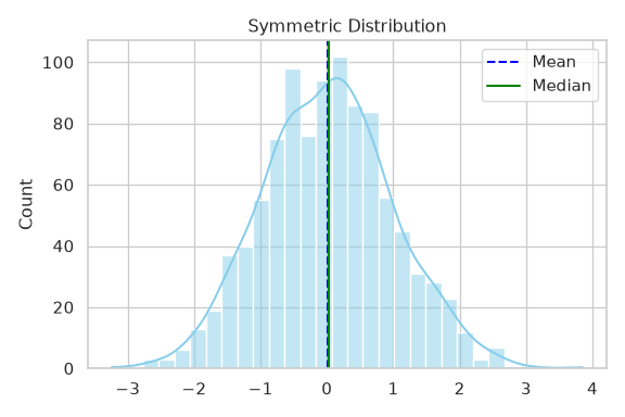
For a symmetric distribution, the mean and the median are equal.
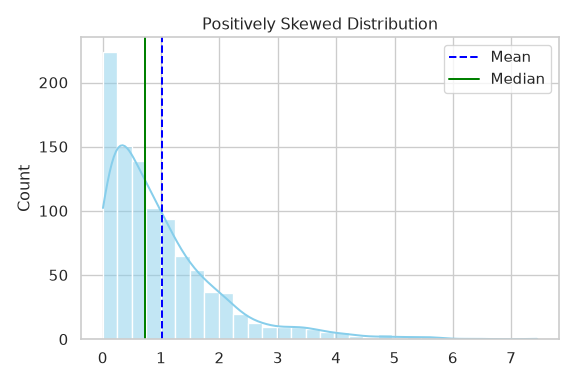
When the data are positively skewed, the mean will usually be greater than the median.
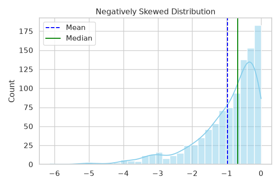
When the data are negatively skewed, the mean will usually be less than the median.
2.3 Z-score
Z-score: The z-score is often called the standardized value. The z-score, \(z_i\), can be interpreted as the number of standard deviations \(x_i\) is from the mean x.
\[z_i = \frac{x_i - \bar{x}}{s}\]
Where:
\[z_i = \text{the z-score for } x_i\]
\[\bar{x} = \text{the sample mean} \]
\[ s = \text{the sample standard deviation} \]
NotePractice problem
A teacher wants to understand how each student’s test score compares to the class average.
A student scored: 92
Class mean (\(\bar{x}\)): 85
Class standard deviation (\(s\)): 5
TipSolution
\[z_i = \frac{x_i - \bar{x}}{s} = \frac{92 - 85}{5} = \frac{7}{5} = 1.4\]
3 Sampling Distributions
In inferential statistics, we want to use characteristics of the sample (i.e. a statistic) to estimate the characteristics of the population (i.e. a parameter).
3.1 Form of the Sampling Distribution of \(\bar{x}\)
The expected value (mean) and standard deviation (standard error) of the sampling distribution of \(\bar{x}\) apply to any population, regardless of its shape.
However, to fully describe the form (or shape) of the sampling distribution, we must consider two cases:
- The population has a normal distribution: If the population is normally (or approximately normally) distributed, then the sampling distribution of the sample mean \(\bar{x}\) is also normally distributed — regardless of sample size 𝑛
→ This means that when sampling from a normal population, even small samples yield a normally distributed sample mean.
- The population does not have a normal distribution: When the population from which we are selecting a random sample does not have a normal distribution, the central limit theorem is helpful in identifying the shape of the sampling distribution of \(\bar{x}\).
NotePractice problem
The researcher collects a random sample of size n = 5.
Is the sampling distribution of the sample mean expected to be approximately normal?
Explain why or why not.
TipSolution
No, because the population is not normal and the sample size is small (n = 5).
Without a normal population, small samples do not guarantee a normally distributed sample mean.
3.2 Central limit theorem
In selecting random samples of size n from a population, the sampling distribution of the sample mean \(\bar{x}\) can be approximated by a normal distribution as the sample size becomes large.
As \(n \rightarrow \infty\), the distribution of \(x_i \rightarrow \text{Normal}\).
In practice, the approximation is usually good when \(n \geq 30\).
This theorem allows us to apply normal probability models even to data from skewed or non-normal populations, as long as the sample size is sufficiently large.
NotePractice problem
Suppose the researcher increases the sample size to n = 40.
How would this affect the shape of the sampling distribution?
What statistical principle supports your answer?
TipSolution
- With n = 40, the Central Limit Theorem applies. The sampling distribution of the sample mean becomes approximately normal, even though the population is skewed.
4 Hypothesis Testing
4.1 Definition of Hypothesis Testing
Hypothesis testing is a fundamental technique in modern statistical analysis, enabling researchers to draw conclusions about populations based on sample data.
It provides a structured approach to assess whether an observed effect is genuinely significant or simply due to random variation.
NotePractice problem
A nutritionist claims that a new diet improves cholesterol levels. To test this, they collect cholesterol readings from a group before and after the diet.
Why hypothesis testing is appropriate in this situation.
TipSolution
- Hypothesis testing is appropriate because it allows the nutritionist to assess whether the observed change in cholesterol levels is statistically significant or could have occurred by random chance.
4.2 Null and Alternative Hypotheses
Hypothesis testing consists of two competing statements about the population: the null hypothesis (\(H_0\)) and the alternative hypothesis (\(H_a\)).
The null hypothesis (\(H_0\)): represents the current assumption, the status quo, or the idea that there is no effect or no difference in a population. It is accepted as true until sufficient evidence suggests otherwise. Examples include:
\(H_0\): The new medication has no impact on blood pressure.
\(H_0\): There is no difference in average income between two groups.
The alternative hypothesis (\(H_a\)) challenges \(H_0\) and expresses the claim the researcher aims to support—suggesting the presence of an effect, difference, or relationship. Examples include:
\(H_a\): The new medication lowers blood pressure.
\(H_a\): There is a difference in average income between the two groups.
These hypotheses shape the foundation of statistical testing. Crucially, we never prove the null hypothesis; instead, we either reject it based on strong evidence or fail to reject it when evidence is insufficient.
This distinction ensures that conclusions remain objective and rooted in probability rather than absolute certainty.
NotePractice problem
A manufacturer wants to test if their new lightbulbs last longer than the industry standard of 1,000 hours.
Formulate the null and alternative hypotheses for this situation.
Indicate whether it is a one-tailed or two-tailed test.
TipSolution
Null hypothesis (\(H_0\)): \(\mu = 1000\) (The average lifespan is equal to 1,000 hours)
Alternative hypothesis (\(H_a\)): \(\mu > 1000\) (The average lifespan is greater than 1,000 hours)
Conclusion: This is a one-tailed test (right-tailed), because the manufacturer is specifically interested in whether the lifespan has increased.
4.3 P-values and Significance Levels
Once hypotheses are established, we need statistical methods to assess whether the evidence supports or contradicts the null hypothesis (\(H_0\)). This is where p-values and significance levels play a crucial role.
4.3.1 Understanding P-value
The p-value represents the probability of obtaining results at least as extreme as those observed in the sample, assuming \(H_0\) is true. In simple terms:
A small p-value (typically ≤ 0.05) suggests that the observed results are unlikely under H₀, indicating stronger evidence against the null hypothesis.
A large p-value suggests that the observed results could reasonably occur if \(H_0\) were true, meaning there is insufficient evidence to reject it.
Mathematically, the p-value is:
\[ \text{p-value} = P(\text{observed data or more extreme} \mid H_0 \text{ is true})\]
4.3.2 Significant level \(\alpha\)
The significant level \(\alpha\) predetermined threshold that dictates when to reject \(H_0\). Common values are: 0.01 (1%); 0.05 (5%); 0.10 (10%).
Rule for reject \(H_0\):
- If \(\text{p-value} \leq \alpha\), reject \(H_0\)
- If \(\text{p-value} > \alpha\), fail to reject \(H_0\)
NotePractice problem
A clinical study tests whether a new vaccine is more effective than the current standard. After analysis, a p-value of 0.03 is obtained. The significance level is set at \(\alpha = 0.05\).
What does the p-value of 0.03 mean in context?
Should the researchers reject or fail to reject the null hypothesis? Why?
TipSolution
The p-value of 0.03 means that if the new vaccine were not more effective (i.e., if the null hypothesis is true), there is only a 3% chance of observing data this extreme.
Since p = 0.03 < α = 0.05, the researchers reject the null hypothesis. There is statistically significant evidence suggesting the new vaccine is more effective.
4.4 Process of Hypothesis testing
4.4.1 Develop Null and Alternative Hypotheses
To formulate hypotheses for a research question, follow these structured steps:
Step 1: Define the parameter of interest—whether it’s a mean, proportion, or difference.
Step 2: Establish the null hypothesis (\(H_0\))—this represents the baseline or “no effect” assumption.
Step 3: Determine the type of test:
Two-tailed: Tests for any difference (≠).
One-tailed: Tests for a specific increase (>) or decrease (<).
Key takeaway
Hypotheses must be mutually exclusive and collectively exhaustive, meaning they cover all possible outcomes.
Significance level (\(\alpha\)) is chosen to determine when to reject \(H_0\); typically 0.05 for most studies.
The test direction (one-tailed or two-tailed) depends on whether you expect a specific change or just any difference.
4.4.2 Determine the Appropriate Test and Execute Analysis
Common statistical tests:
| Test Type | Application | Assumptions |
|---|---|---|
| Z-test | Testing means, known population variance | Normal distribution or large n, known population standard deviation |
| T-test | Testing means, unknown population variance | Normal population (or large sample), unknown population variance, continuous data |
| Chi-square test | Testing categorical data (goodness-of-fit or independence) | Large sample, expected frequency > 5 in most cells |
After selecting the appropriate test, executing the analysis involves:
Checking that your data meets test assumptions
Calculating the test statistic
Determining critical values or p-values
Making a statistical decision
NotePractice problem
Choose the correct hypothesis test:
You want to compare the mean GPA of students in two different colleges, and population variance is unknown.
You want to test if the observed gender ratio in a class (40 male, 60 female) differs from the expected 50:50.
You want to test if the average daily sales of a store differ from $500, with a known standard deviation.
Answer format: a: ____, b: ____, c: ____
TipSolution
a: T-test (comparing means, variance unknown)
b: Chi-square test (categorical data — goodness-of-fit)
c: Z-test (mean, population standard deviation known)
4.4.3 Interpret the Statistical Results
A well-rounded statistical interpretation involves several key components:
Statistical decision: Determine whether to reject or fail to reject the null hypothesis (\(H_0\)) based on the significance level (\(\alpha\)) and p-value.
Context: Explain what this decision means in relation to your research question—whether the observed effect supports a meaningful claim.
Effect size: Assess the magnitude of the difference or relationship, ensuring it is practically important, not just statistically significant.
Confidence intervals: Identify the range of plausible values for the parameter, offering a measure of precision in the estimate.
Limitations: Recognize potential influences on validity, such as sample size, biases, or external factors that may affect generalizability.
NotePractice problem
A two-tailed t-test is conducted at \(\alpha = 0.05\) to test whether a new fertilizer changes plant growth. The p-value is 0.12, and the 95% confidence interval for the mean difference is (–1.2 cm, 0.5 cm).
What statistical decision should be made?
What does this decision imply in the context of the experiment?
Is the effect practically significant? Justify your answer using the confidence interval.
TipSolution
Fail to reject the null hypothesis (since p = 0.12 > 0.05).
There is insufficient statistical evidence to conclude that the fertilizer changes plant growth.
The effect is not practically significant because the confidence interval includes 0, and the range (–1.2 cm to 0.5 cm) suggests any change is small and could even be negative.